|
Interacting Systems: Hidden Complexity in Nature
P. F. Allport
To understand nonliving and living things and how they evolved
into their present forms, we need to understand how systems of matter interact.
The evolving matter is in the form of atoms, molecules, cells and
larger-scale systems of these building blocks including minerals, animals, populations of animals,
environments, planets, stars, and galaxies. Interactions between systems of matter determine
heart rates, cultural changes in societies, economic booms and busts, natural disasters and other
events in and around us, so it's useful to have an awareness of interacting systems.
The history of science has been a history of improved understanding of how systems in nature interact.
Simple mathematical models
To study interacting systems, the systems and interactions can be represented mathematically.
Newton and other scientists used mathematical modeling to help
understand how planets orbit the sun, how populations of
animals change in response to changes in their environments, and why various forms of matter evolved
into the configurations found in nature.
We will discuss several mathematical models of interacting systems that show surprising features
of simple feedback processes.
We will start with an interaction between two systems. Each system evolves in
a way that depends on the current values of the systems, much like a population
of animals and the animals' environment
evolve in ways that depend on both the current state of the population and the current state
of the environment. The evolution of the two systems, P and E, is defined mathematically as follows, where n
means the nth step (i.e. step number n) in a step-and-repeat (i.e. recursive) process in
which the two systems evolve.
P = P = P + E
− 1.25
E = E − P + E
− 1.25
E = E − P
 |
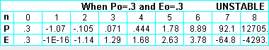
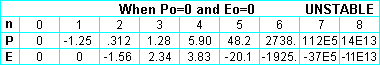
For some combinations of initial values for P and E the interaction is unstable. For example, if we
start with Po=.3 and Eo=.3 (middle table) or
Po=0 and Eo=0 (bottom table),
we find that P and E quickly become large positive
or negative values and eventually become infinite. Therefore, the starting values of P and E determine
whether or not the interaction is stable. We can determine what combinations of starting values of
P and E result in stable interactions by systematically trying different combinations of
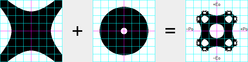
starting values. The Holes pattern above is the result of trying 201
combinations of starting values of P, from −2 at the left end of the horizontal axis to +2 at the
right end, and 201 combinations of starting values of E, from −2 at the bottom of the vertical axis
to +2 at the top. Therefore, the pattern shows 40401 combinations of Po and Eo,
and each combination is represented by a dot or pixel on the pattern. White pixels show where the combinations
of Po and Eo result in instability, and black pixels show where
the Po,Eo combinations result in stable interactions.
The grid lines on the pattern appear every .5 units.
The Holes pattern is symmetrical around horizontal, vertical, and diagonal axes.
Around the center hole are four secondary holes, eight tertiary holes, sixteen quaternary holes, thirty-two
quinary holes, etc., and this doubling at each smaller scale results in an infinite number of holes.
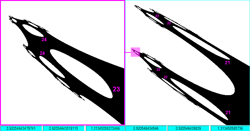
Appendix I (at end of document) shows the Holes pattern at a location where the doubling has occurred
about 25 times, so the number of holes of the sizes shown is over a million. The Holes process shows that even
simple systems can interact in ways that result in complex patterns of stability.
Natural processes reflect characteristics of the interacting systems
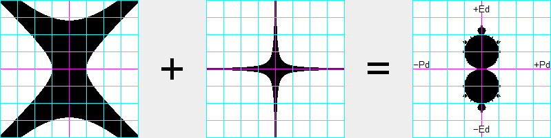
The Holes pattern reflects characteristics of the two systems that interact to create the pattern.
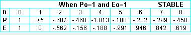
It reflects the X-shape pattern above-left that we get if we replace the first equation above with P=1 so
P is always 1 during the interaction.
And it reflects the above-center pattern of stability and hole of instability that we get if we replace
the second equation with E=1 so E is always 1.
If the constant 1.25 is decreased to a number greater than 1, the holes in the center pattern and Holes pattern
become smaller, and if the constant is decreased to 1, all the holes disappear.
Like many kinds of interacting systems in nature,
each system can influence the characteristics of the resulting interaction. And systems found
in nature generally exist because they have been able to survive in combination with other systems. They
have evolved characteristics that allow them to survive in stable interactions with other systems. The patterns
on this web page, like all forms of matter we see, are the result of very complex processes. It's easy
to see the patterns and forms of matter, but difficult to understand the causes that occur behind the scenes.
Perfect Diamond process
Another two-system interaction or process that has interesting characteristics is specified by the P and E
equations below. In this process Po and Eo are always zero, and the
stability of the process depends on "disturbances" Pd and Ed that influence the values of
P and E during each step of the interaction. At any point or pixel on the stability pattern, Pd is
equal to the distance from the Ed axis to the point, and Ed is equal to the distance from the Pd axis to the point.
An example will make this clearer.
P = (Pn+Pd)(En−Ed) + (Pn−Pd)(En+Ed)
E = (En+Ed)(En−Ed) + (Pn+Pd)(Pn−Pd)
 |
|
Let's see how these two systems interact if we select the point at the center of our plot where Pd=0 and Ed=0
(the distances in the Pd and Ed directions respectively). In this case P1=0
and E1=0 because Po and Eo are zero and because
disturbances Pd and Ed are zero.
Therefore, P and E stay at zero during every step of this very stable-but-boring interaction of the two systems.
When Pd=.5 and Ed=.5, the process is also stable but a little less boring because
P and E both evolve as follows: 0, −.5, 0, −.5, 0, −.5, etc.
When Pd=1 and Ed=1, the interaction is unstable and
P and E both evolve as follows: 0, −2, 6, 70, 9798 ... and become infinite.
When Pd and Ed are unequal, P and E evolve differently. For example, if Pd=0 and Ed=1 (or if Pd=1 and Ed=0)
then P=0 throughout the interaction and E oscillates back and forth from 0 to −1.
And when Pd=0 and Ed=1.2 (or when Pd=1.2 and Ed=0) then P stays at zero but E oscillates in a range from about
−1.44 to about 0.64.
|

|
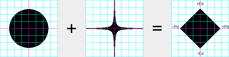
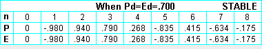
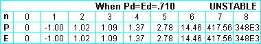
What is the interaction near the midpoint of the upper right edge of the diamond?
When Pd=.700 and Ed=.700, then P and E are always the same and they oscillate in a range from −.98 to about .94, as shown in top
table above. But when Pd=.710 and Ed=.710, then the interaction is unstable, and P and E both evolve as shown in the
bottom table. The transition between stability and instability occurs when Pd and Ed equal the square root of .5 or .707106781... ,
in which case P and E both evolve as shown in the middle table.
In spite of the variety of interactions, the resulting pattern of stability is a perfect diamond that is symmetrical about the Pd, Ed
and diagonal axes of the coordinate system. It has square corners and sides exactly 1 unit long. At every point along the
four edges of the diamond the interaction between the P and E systems evolves so that P+E=2 or −P+E=2.
Duality process
The following two-equation interaction or process is like the perfect diamond process except that the
E equation has a minus sign between the E and P terms and it has the +.25 constant. This process results in the
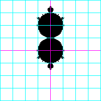
"Duality" pattern of stability, which has characteristics in common with Julia and Mandelbrot patterns.
Like Julia patterns it has two identical halves. Attached to these two identical subpatterns are similar,
smaller-scale versions, to which are attached still-smaller subpatterns, etc. Due to the balanced disturbances
in the Duality process, the stability pattern is symmetrical about both the Pd and Ed axes.
P = (Pn+Pd)(En−Ed) + (Pn−Pd)(En+Ed)
E = (En+Ed)(En−Ed) − (Pn+Pd)(Pn−Pd) + .25
 |
|
The pattern's two main discs are exactly 1 unit in diameter. Within these main discs, the outcome of the interaction
process is easily predictable by the following rule. Rule: For any point within the
upper main disc, the variable P converges to (i.e. homes in on) −Pd, and E converges to (.5−Ed);
and for any point within the lower main disc, P converges to +Pd and E converges to (.5+Ed).
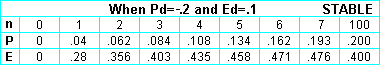
We can check this rule by selecting a combination of values for Pd and Ed and then see how the Duality process evolves.
We will let Pd=−.2 and let Ed=+.1, which is a combination in the upper main disc. The interaction evolves as
shown in the first table under the Duality pattern. After 100 interactions, P=.200
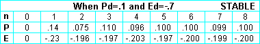
and E=.400 as specified by the above Rule. And in the lower disc we can try Pd=.1 and
Ed=−.7 as shown in the second table. After 100 interactions P has converged to Pd and E has converged
to .5 plus Ed, as specified by the Rule.
|
|
The following image shows the Duality pattern of stability (gray) bounded
by areas of increasing instability (white through colors to white background). It also shows the horizontal lines of constant
values of E to which E converges and the vertical lines of constant values to which P converges. These iso lines
(i.e. lines of equal P or equal E) are spaced .05 units on centers. The animation (below-left) shows how these
isoP and isoE lines change during the first 1, 2, 4, 8, 16, etc. interactions of the P and E systems. The straight
iso lines within the primary area of stability may be a unique characteristic of the Duality process.
|
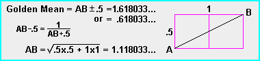
Golden Mean (GM) and the Duality process
(GM=.6180339887498948482045868343656...)
When Pd=0, some values of Ed result in what we call "perfect processes." For example, when Pd=0 and
Ed=±.5, the value of E never changes from zero as the Duality systems interact. In this case E
stays at a single value, zero. A perfect process also occurs at the two values of Ed that result in E always being
one of two numbers. The values of Ed where this occurs are
±(.5+GM) or ±1.118033... or ±(square root of 1.25),
as shown in the figure at right.
(If you are unfamiliar with the Golden Mean, it is a fascinating ratio that is
explained at several excellent websites and videos including
this one and
this one.)
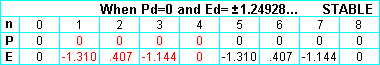
When Ed=±1.118033..., E is either 0 or −1, as shown
in the first table at right. A perfect process also occurs at
Ed=±1.24928..., as shown in the second table. In this cases E is always one of four numbers,
as shown. The sequence of values of E during the first four steps of the process is exactly the same as the sequence
during steps 5 through 8 and steps 9 through 12, etc. Similarly, there are perfect processes where E is always one of
eight numbers, and perfect processes where E is always one of sixteen numbers, 32 numbers, 64 numbers, etc.
Appendix II a shows golden rectangles resulting from the perfect processes.
|

|
Within Duality's main discs, P and E each converge to a single number, as we have seen. In the secondary discs atop the
main discs P and E each converge to two numbers, and in the discs atop the secondary discs P and E each converge to
four numbers, etc. Thus in the 30th disc out from a main disc P and E each converge to a sequence of over a billion numbers,
and the sequence keeps repeating over and over during the process. This is an
example of the complexity found in this mathematical process.
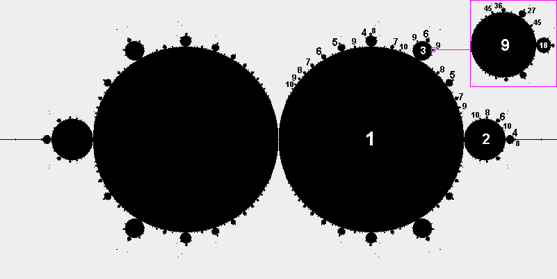
Appendix II b shows the self-similarity on all scales and the increasing complexity of the interactions at
smaller scales.
The numbers in the discs show the number of values in the sequence of numbers to which the variables converge for
all Pd,Ed combinations in the disc. For example, for all locations in the main disc with number 1, P and E each
converge to 1 value, as discussed above. And everywhere in little disc number 9, that has been enlarged,
P and E each converge to a sequence of nine values. A simple rule allows one to determine the number of values in
the sequence for any disc. You can probably determine the rule from the numbered discs on the pattern.
Natural process approximations to perfect mathematical processes
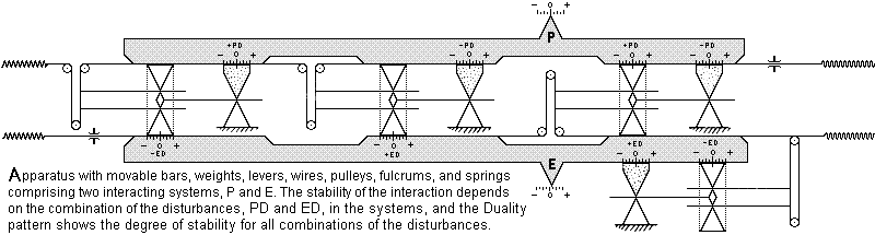
The Duality process can occur with various interacting systems including the mechanical systems in the apparatus diagramed
below. This apparatus, like evolving mechanical, biological, chemical, and atomic processes, is a calculator.
The values of P and E that the moveable P and E bars indicate on the top and bottom scales depend on the previous positions
of the bars and the positions of the four weights and four fulcrums that are adjusted automatically or manually at every
step of the step-and-repeat process. If we carefully constructed and used this apparatus to determine what combinations of
Pd and Ed result in stable evolution of P and E, the results would allow us to plot a crude Duality pattern.
Natural processes tend to be crude approximations of ideal processes. Conversely, mathematical processes represent
unrealistic perfect processes that are not found in nature. Clock technologies provide examples.
Early mechanical clocks were inaccurate because they did not evolve like the
theoretical clocks represented by the clocks' designs. Atomic clocks are much more accurate because they are
based on subatomic processes where the natural consistency is close to the theoretical consistency.
|
Duality process with Pd axis through center of bottom main disc
The following two-equation interaction is a variation of the Duality process above. The .25 constant has
been removed from the E equation, and disturbances Pd and Ed have been added to the P and E equations respectively,
as shown. These changes shift the pattern upward .5 units in the coordinate system so the Pd axis passes through the
center of the bottom main disc. The centers of the main discs are now at Ed=0 and Ed=1, two numbers that do not change
regardless of the powers to which they are raised.
P = (Pn+Pd)(En−Ed) + (Pn−Pd)(En+Ed) + Pd
E = (En+Ed)(En−Ed) − (Pn+Pd)(Pn−Pd) + Ed
|
|
Duality transformations
By modifying the Duality equations and unbalancing the disturbances, the pattern of stability can be changed in many ways.
The changes usually cause a loss of symmetry or other characteristics that make Duality special.
The pattern can be changed into Julia and Mandelbrot patterns, as shown in the following animations.
About this project
Back when CPM was a popular computer operating system, a friend introduced me to personal computers.
This was a huge help because I had been using a calculator and graph paper to determine how various systems interact.
With a computer I could quickly plot patterns of stability and cellular automata growth patterns.
The above processes are some of the results of my continued interest in interacting systems. A study of different
kinds of disturbances in the systems in 1988 resulted in finding the Duality process. This process seemed to have
extraordinary characteristics so I described it in documents that I copyrighted and sent to several journals
including Byte, Physics Today, and Nature where articles on chaos theory and fractals had appeared.
The information was not published and I have not tried other submissions. Duality appears in What Is Life?
by Lynn Margulis and Dorion Sagan. A purpose of the above information is to encourage interest in the role of
interacting systems in shaping everything in nature. The hidden complexity in nature has long led to false ideas.
It led to false ideas about the sun, rain, lightning, diseases, intelligence, and a variety of other complex
phenomena. Understanding how simple systems can interact in complex ways helps one understand the complexity found
in ourselves and our environments. Realizing that diamonds, snowflakes, microbes, galaxies, and other highly
organized or complex forms of matter are natural consequences of interacting systems of matter helps make
nature less perplexing.
© 1989-2009 by P. F. Allport.
Appendix I
Holes stability pattern at Po=.920546435 and Eo=1.313450583
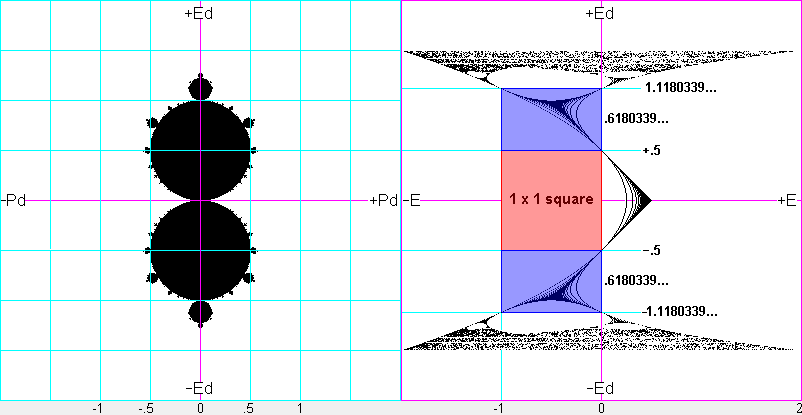
Appendix II a
Duality (below-left) and Plot of E for Ed from −2 to +2 when Pd=0 (below-right). The plot shows the
perfect processes at Ed=±.5 and Ed=±1.1180339..., and shows the
resulting golden rectangles (blue) and larger-scale golden rectangles formed by each of the
blue rectangles plus the 1x1 square.
Appendix II b
Duality stability pattern (with Ed axis horizontal) showing self-similarity on all scales and
increasingly complex process at smaller scales.

Interacting Systems: Hidden Complexity in Nature by Peter F. Allport is licensed under a
Creative Commons Attribution-Noncommercial-Share Alike 3.0 United States License.
For additional information contact info@qmview.net
|